
Mathedu Courses
Mathedu Courses
If you see this, something is wrong
First published on Thursday, Sep 3, 2026 and last modified on Saturday, Sep 5, 2026
The course of linear algebra we enter into starts with a discovery of the systems of linear equations both in their matrix view as for their nice applications in the real world.
We will start that course of linear algebra with the solutions of two systems of linear equations.

A plane travelling
Assume that a plane travels between two cities separated by a distance of 5,000 km.
Assume that the trip one way against a headwind takes \( 6 \frac{1}{4}\) hours, and that the return trip the same day in the direction of the wind takes only \( 5\) hours.
Then you must find the ground speed of the plane and the speed of the wind, assuming that both remain constant.
Let \( x\) represent the speed of the plane in km/h and \( y\) the speed of the wind in km/h.
Then the following equations model the problem.
Consequently, we have to solve the system of two linear equations in two real variables:
(1)
If we replace the second equation by itself minus the first equation, we obtain:
(2)
that is equivalent to
(3)
The first equation is then equivalent to:
(4)
that is equivalent to
(5)
The solution of the problee of the plane is thus:
The following Python script allows us to visualize the equations of the system 1 as straight lines in the plane and the solution at a big dot at the intersection of the two lines.
from numpy import *
from matplotlib.pyplot import *

×=arange(-100,2000,100)
y1=x-800
y2=1000-x

plot(x,y1,'b',label='Equation1')
plot (x,y2, 'r', label= 'Equation 2')
plot(900,100, 'ko', markersize=5, label=' Solution')

legend()
grid()
The figure it draws is the following.
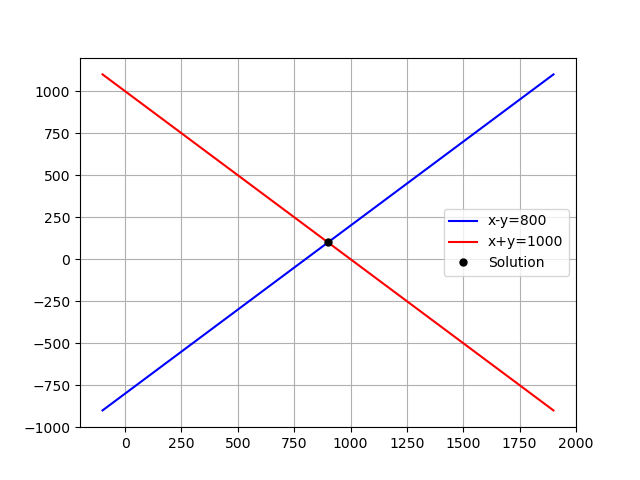
Graphical solution of a linear system
We will now try to find a parabola that passes through three points of the plane.
We want to determine the polynomial \( P(x)=a_0+a_1x+a_2x^2\) whose graph passes through the points \( (1,4)\) , \( (2,0)\) , and \( (3,12)\) .
The polynomial \( P(x)\) must then be such that:
\( P(1)=4\) , \( P(2)=0\) and \( P(3)=12\) .
If we substitute \( 1\) , \( 2\) and \( 3\) to \( x\) into \( P(x)\) , we obtain:
We thus have to solve the following system of linear équations in the variables \( a_{0}\) , \( a_{1}\) and \( a_{2}\) .
(6)
Subtracting the first equation to the second and third equations gives:
Then subtracting 2 times the second equation to the third equation gives:
The last system is a system in row echelon form, with the coefficients below the main diagonal reduced to \( 0\) .
Let’s solve it by back substitution.
The searched polynomial is thus \( P(x)=24-28x+8x^{2}\) .
The following Python script illustrates the fact that tha graph of the polynomial \( P(x)=24-28x+8x^{2}\) passes through the points \( (1,4)\) , \( (2,0)\) , and \( (3,12)\) .
from numpy import *
from matplotlib.pyplot import *

x=arange(-2,6,0.01)
y=24-28*X+8****2

plot(x,y,'b',label='$y=24-28x+x^2$')

plot(1,4, 'ko',markersize=5)
plot(2,0, 'ko',markersize=5)
plot(3,12, 'ko',markersize=5)

grid()
legend(
The figure it draws is the following.
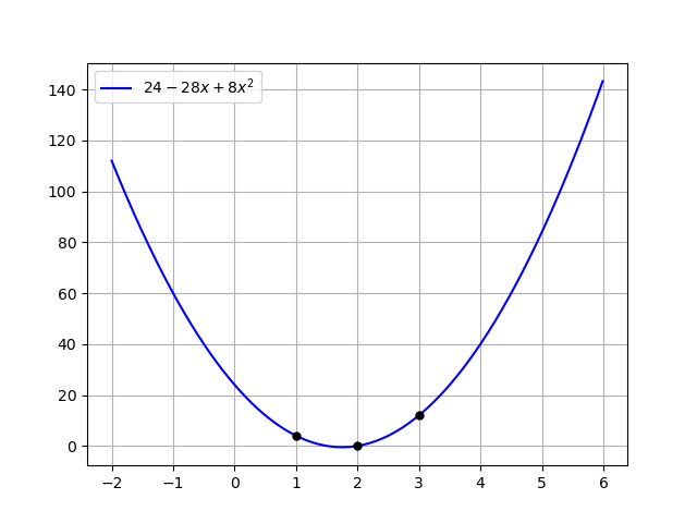
Polynomial Fit
Plane travelling
Consider the system 1:
and consider the matrix and the vectors:
The result of the matrix multiplication of \( A\) and \( X\) is
\( AX=\begin{bmatrix} 1&-1\\ 1&1 \end{bmatrix} \begin{bmatrix} x\\ y \end{bmatrix} =\begin{bmatrix} x-y\\ x+y \end{bmatrix}\) , where:
Let’s note that the elements of \( AX\) are the left members of the equations of the system 1.
Consequently, the linear system 1 is equivalent to the matrix equation
\( AX=B\) .
A system of \( m\) linear equations in \( n\) real variables is a set of equations of the form:
(7)
where \( a_{ij}\in\mathbb{R}\) is the coefficient of \( x_{j}\) in the \( i\) -th equation and \( b_i\) is the second member of the \( i\) -th equation.
By definition, a solution of the sytem 7 is a \( n\) -uple of real numbers
\( (x_{1},x_{2},…,x_{n}\in\mathbb{R}^{n}\) such that all the equations of the system are verified for these real numbers.
And solving the system 7 is finding all the solutions, if any, of that system.
We will discover later in the course that the set of solutions of a system of linear equations is of one of these kinds:
For the system 7, we consider the followin matrix and vectors:
An important other matrix to solve linear systems is the augmented matrix \( \overline{A}\) , made of the coefficients matrix \( A\) with the second members colum vector \( B\) in its last column:
The result of the matrix multiplication of \( A\) and \( X\) is
\( AX=\begin{bmatrix} a_{00}&a_{01}&…&a_{0,n-1}\\ a_{10}&a_{11}&…&a_{1,n-1}\\ \vdots&\vdots&&\vdots\\ a_{m-1,0}&a_{m-1,1}&…&a_{m-1,n-1}\\ \end{bmatrix} \begin{bmatrix} x_0\\ x_1\\ \vdots\\ x_{n-1} \end{bmatrix} =\begin{bmatrix} a_{00}x_0&+&a_{01}x_1&+&…&+&a_{0,n-1}x_{n-1}\\ a_{10}x_0&+&a_{11}x_1&+&…&+&a_{1,,-1}x_{n-1}\\ \vdots&&\vdots&&&&\vdots\\ a_{m-1,0}x_0&+&a_{m-1,1}x_1&+&…&+&a_{m-1,n-1}x_{n-1} \end{bmatrix} \) , where:
Let’s note that the \( m\) elements of \( AX\) are the left members of the \( m\) equations of the system 1.
Consequently, the linear system 7 is equivalent to the matrix equation
\( AX=B\) .
The following Python script solves a sqaure linear system of \( 10\) equations in \( 10\) unknowns and checks graphically the the column vector \( X\) obtained is indeed a solution.
The coefficient matrix and the second members column vector are made of random elements and the solution of the linear system is a call to the numpy.linalg function ‘X=solve(A,B)’ that solves in fact the matrix equation \( AX=B\) .
The function ‘iùshow(M)’ of ‘matplotlib.pyplot’ allows to visualize matrices and column vecors. We use it to visualize the coefficients matrix \( A\) check that the output ‘X’ of ‘solve(A,B)’ is indeed a solution of the matrix equation\( AX=B\) .
from numpy import *
from numpy.linalg import *
from matplotlib.pyplot import *

A=random.randn(10,10)
imshow(A)
title('coefficients matrix A')

B=random.randn(10,1)
X=solve(A,B)

figure()

subplot(1,2,1)
imshow(B)
title('second members B')

subplot(1,2,2)
imshow(A@X)
title('product AX')
The figures it draws are the following.
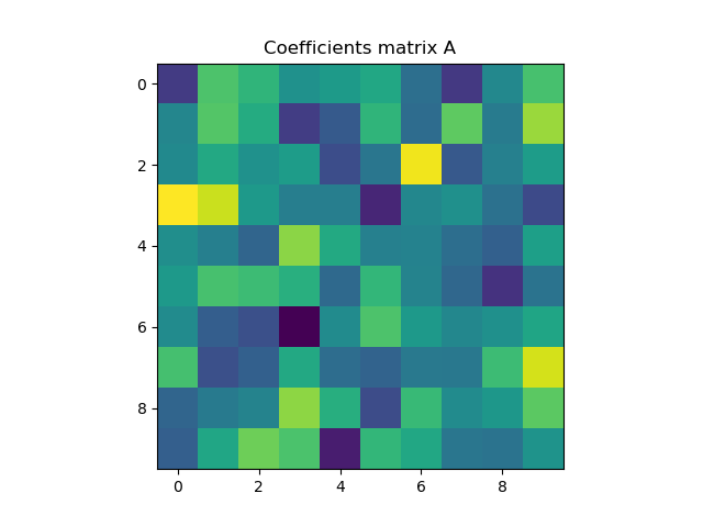
The coefficient matrix
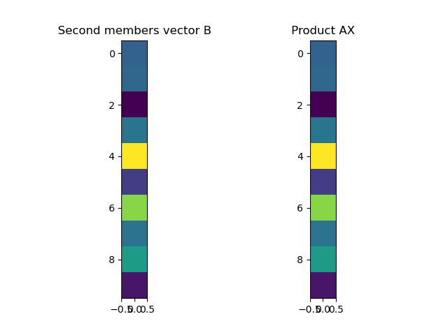
Solution check
Note that the details of the colors defere from run to run of the script, because the matrix \( A\) and the column vector \( B\) contain random numbers.
The important thing is that on the second figure, the column vectors \( B\) and \( AX\) are the same.
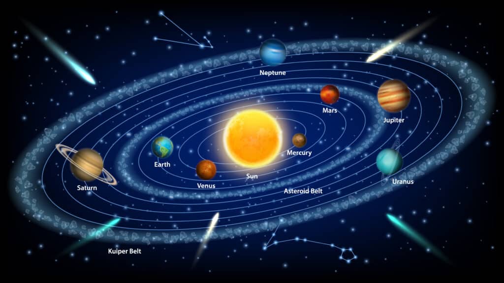
The solar system
And now we shall apply the linear systems to the discovery of the third Kepler law for the planets of the solar system that relates their mean distances to the sun to their period.
The table 1 below gives the mean deistances to the sun and the periods of the first six planets of the solar system.
The distances are measured in astronomical units, a,d the periods are measured in years.
| Planets | Mercury | Venus | Earth | Mars | Jupiter | Saturn |
| Distance (%) | \( 0.387\) | \( 10.723\) | \( 1.0\) | \( 1.523\) | \( 5.203\) | \( 9.541\) |
| Period (%) | \( 0.241\) | \( 0.615\) | \( 1.0\) | \( 1.881\) | \( 11.861\) | \( 29.457\) |
We want to fit a quadratic polynomial to the data of the first three planets, Mercury, Venus and the Earth.
Hence we want to find a ploynomial \( P(x)=a_0+a_1x+a_2x^2\) which graph passes throught the points \( (0.287,0.241)\) , \( (0.723,0.615)\) and \( (1.0,1.0)\) .
As we saw in the § 6, this is equivalent to solving the linear system in \( a_{0}\) , \( a_{1}\) and \( a_{2}\) :
(8)
After doing that in Python, we will check the solution for the next three planets, Mars, Jupiter and Saturn, again in Python.
The following Python script solves the polynomial fit problem, visualizes it for the first three planets and for Mars and calulates the errors for Mars, Jupiter and Saturn.
from numpy import *
from numpy.linalg import *
from matplotlib.pyplot import *

# Distances of the planets to the sun in AUs
Dist=array([0.387,0.723,1.0,1.523,5.203,9.541])

# Coefficients matrix
A=array([[1.0,Dist[0],Dist[0]**2],
        [1.0,Dist[1],Dist[1]**2],
		[1.0,Dist[2],Dist[2]**2]])
print('the coeeficients matrix is A=\n',A)

# Periods of the planets in years
Period=array([0.241,0.615,1.0,1.881,11.861,29.457])

# Second members column vector
B=array([[Period[0]],[Period[1]],[Period[2]]])
print('The second members column vector is B=\n',B)

# The polynomial that fits the three first planets data
a=solve(A,B)
a0=a[0,0]
a1=a[1,0]
a2=a[2,0]
print('The polynomial is\n',a0,'+',a1,'x+',a2,'x^2')

# Visualisation
x=arange(0,2,0.01)
y=a0+a1*x+a2*x**2
plot(x,y,label='the parabola')
# Mercury
plot(Dist[0],Period[0],'ko',markersize=3)
# Venus
plot(Dist[1],Period[1],'ko',markersize=3)
# Earth
plot(Dist[2],Period[2],'ko',markersize=3)
grid()
legend()

#Check
# Mars
plot(Dist[3],Period[3],'ko',markersize=3)
P_of_Mars=a0+a1*Dist[3]+a2*Dist[3]**2
print('The error for Mars is ',Period[3]-P_of_Mars)
# Jupiter
P_of_Jupiter=a0+a1*Dist[4]+a2*Dist[4]**2
print('The error for Jupiter is ',Period[4]-P_of_Jupiter)
# Saturn
P_of_Saturn=a0+a1*Dist[5]+a2*Dist[5]**2
print('The error for Saturn is ',Period[5]-P_of_Saturn)
The figure it draws is the following.
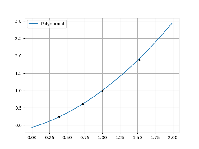
The first 3 planets are on the graph, but not March.
You can see that the first three planets ore on the graph of the polynomial, but not Mars.
The error for mars is several days, and the errors for the other planets become greater as the ir distance to the sun enlarges.
Consequently, the polynomial fit for the first three planets doesn’t allow extrapolation to further planets. But you will see that taking tha natual logarithms of the data allows a linear fit for all the six planets.
We will see in Python that the natural logarithms of the data allow linear fit with the straight line of equation \( Y=\frac{3}{2}X\) .
The previous Python script is enriched with the following lines to show that graphically.
# Fitting the natural logarithms with a straight line
LnDist=log(Dist)
LnPeriod=log(Period)
X=arange(-2,4,0.01)
Y=(3/2)*X

figure()
plot(X,Y,label=('The straight line'))
# Mercury
plot(LnDist[0],LnPeriod[0],'ko',markersize=3)
# Venus
plot(LnDist[1],LnPeriod[1],'ko',markersize=3)
# Earth
plot(LnDist[2],LnPeriod[2],'ko',markersize=3)
# Mars
plot(LnDist[3],LnPeriod[3],'ko',markersize=3)
# Jupiter
plot(LnDist[4],LnPeriod[4],'ko',markersize=3)
# Saturn
plot(LnDist[5],LnPeriod[5],'ko',markersize=3)
grid()
legend()
The new figure the completed script draws is the following.
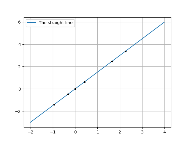
The logarithms of the data are aligned
You may see that the data of all the six planets are align and on the straight line of equation \( Y=\frac{3}{2}X\) .
If \( D\) is the distance to the sun of a planet and \( P\) is its period, then they are related to one another with the formula:
\( Ln(P)=\frac{3}{2}Ln(D)\) , that is equivalent to \( Ln(P^2)=Ln(D^3)\) .
Consequently, there exists a constant \( K\) depending on the measurement units such that \( P^2=KD^3\) .
So that the square of the period of a planet is proportional to the cube of its distance to the sun.
This is the third Kepler law for the planets of the solar system.
The general formulation of that law for any orbital system is:
The ratio of the square of an object’s orbital period with the cube of the semi-major axis of its orbit is the same for all objects orbiting the same primary.
We have discovered in that entry text of our course of linear algebra that the systems of linear equations are usefully represented as a matrix equation that may be solved in one line in Python.
And we had a glance to the numerous applications of such systems in the real world.